2.4 - Sentiment analysis of dreams
By Christian Ryan
February 15, 2020
In the last post we compared the dream sets by graphing the most frequently occurring words and calculating correlation coefficients. But in psychology, we are often interested in specific aspects of the text to analyse. From my own perspective, emotional language use is of particular interest. A further way in which we could compare the dreams is by carrying out a sentiment analysis. One could use bespoke software such as the LIWC programme ( http://liwc.wpengine.com) in this scenario, but the tidytext approach allows for more flexibility, even if the dictionaries are not as well validated as LIWC.

There used to be three sentiment dictionaries included in the tidytext package and the current version of Text mining with R ( https://www.tidytextmining.com) describes them this way. However, some changes have happened to the package, and now it comes with only the Bing set preloaded. To access the other lexicons, we need to install the textdata package.
install.packages("textdata")
Then we load it into the library and run the lexicon_afinn() function. This creates a pop-up in the console which we need to respond to, confirming we wish to download the lexicon. Here I have stored it as a new tibble called afinn.
library(textdata)
library(tidyverse)
afinn <- lexicon_afinn()
Let’s reload our data from the previous post.
load("df_word.Rdata")
Before we get started, we will load some other packages into the library that we might need.
library(tidytext)
library(car)
We can have a quick view of the lexicon by using the some() function from the car package.
some(afinn)
## # A tibble: 10 × 2
##    word       value
##    <chr>      <dbl>
##  1 astounded      3
##  2 bamboozled    -2
##  3 criticize     -2
##  4 drag          -1
##  5 infatuated     2
##  6 mongering     -2
##  7 redeemed       2
##  8 skepticism    -2
##  9 toothless     -2
## 10 trapped       -2
Here we see the various ratings given for the valence of each word regarded as having sentiment. This is scored on a scale from -5 to +5.
Merging sentiment with dream dataset via inner_join()
As we have our original data as df_word and the new dataframe afinn, we can use the inner_join() which will join the two datasets together, keeping only those rows that match. There is a word variable in both datasets, so this value will be used automatically as the *by = * argument for the join. We could have been explicit and written inner_join(afinn, by = “word”), but we know that both datasets contain a word variable so we can skip this step, and you will notice we get a message confirming this is how the join was made.
df_word <- df_word %>%
  inner_join(afinn)
## Joining, by = "word"
df_word
## # A tibble: 1,921 × 4
##    sample        dream_number word     value
##    <fct>                <int> <chr>    <dbl>
##  1 college_women            2 dream        1
##  2 college_women            3 failed      -2
##  3 college_women            4 careful      2
##  4 college_women            5 dream        1
##  5 college_women            5 straight     1
##  6 college_women            5 laughing     1
##  7 college_women            5 stopped     -1
##  8 college_women            6 angry       -3
##  9 college_women            6 dream        1
## 10 college_women            7 hard        -1
## # … with 1,911 more rows
After matching words in the afinn sentiment lexicon with words in our dreams dataframe df_word, we can run a count to see the most frequently occurring words with sentiment ratings. If we also group_by the word and value, we can see the sentiment assigned to each word at the same time. We will use a trick I learned from David Robinson’s video “Ten Tremendous Tricks in the Tidyverse” which is here.
https://www.youtube.com/watch?v=NDHSBUN_rVU
He points out that the count() function has a name argument so we can assign it a name rather than the default of “n”. Here we will call it frequency as it is representing the frequency of words by token.
df_word %>%
  group_by(word, value) %>%
  count(word, sort = TRUE, name = "frequency")
## # A tibble: 591 × 3
## # Groups:   word, value [591]
##    word      value frequency
##    <chr>     <dbl>     <int>
##  1 dream         1       132
##  2 leave        -1        43
##  3 feeling       1        34
##  4 dead         -3        31
##  5 happy         3        28
##  6 top           2        28
##  7 stop         -1        27
##  8 beautiful     3        26
##  9 stopped      -1        24
## 10 afraid       -2        22
## # … with 581 more rows
We can see that the word “dream” is the most frequently occurring word in the dataset with a sentiment rating. For a research study we would need to decide how to treat the word dream in this context. Should it be added as a custom stop-word? We might think of the valence rating as wrong in this context, as the afinn dictionary is almost certainly giving a “1” value for the use of the word in common parlance in which it is used to refer to future plans - “I dream I will get married”; “I dream of winning the lottery”. These kind of wish fulfilment thoughts are probably mildly positive. However, the vast majority of uses of the word dream in this dataset is in a purely functional manner “I was dreaming that…”, which is probably neutral in terms of valence. We could regard occurrence of the word “dream” in the lexicon as an artefact when reporting the content of a dream, and justify removing it from the sentiment analysis. However, for simplicity, and as it only has a valence of ‘1’, we will leave it in.
If we include the ‘sample’ as the first argument of the count() function, we can retain this variable in the output. Then if we give our group_by() function the arguments for word, value and dream_number, we can separate out the word and the sentiment (value) for each dream_number. The difference here is that we are counting the most frequent sentiment words per dream rather than per sample. We will come back to this issue of level of analysis later in this post as we look at ways to aggregate the sentiment.
df_word <- df_word %>%
  group_by(word, value, dream_number) %>%
  count(sample, word, sort = TRUE, name = "frequency")
df_word
## # A tibble: 1,731 × 5
## # Groups:   word, value, dream_number [1,731]
##    word    value dream_number sample        frequency
##    <chr>   <dbl>        <int> <fct>             <int>
##  1 crying     -2          305 hall_female           4
##  2 dead       -3          336 hall_female           4
##  3 dream       1          258 hall_male             4
##  4 hide       -1          202 hall_male             4
##  5 top         2          322 hall_female           4
##  6 war        -2          113 vietnam_vet           4
##  7 barrier    -2          173 vietnam_vet           3
##  8 blocks     -1           65 college_women         3
##  9 crying     -2          381 hall_female           3
## 10 dead       -3          351 hall_female           3
## # … with 1,721 more rows
Here we see that ‘crying’ occurred 4 times in one dream (number 305), as did ‘dead’ and ‘war’.
Strongest sentiments
We could also look at arranging the data just by values. What are the most positive words that occurred in the dream dataset?
df_word %>%
  arrange(desc(value))
## # A tibble: 1,731 × 5
## # Groups:   word, value, dream_number [1,731]
##    word      value dream_number sample      frequency
##    <chr>     <dbl>        <int> <fct>           <int>
##  1 superb        5          157 vietnam_vet         1
##  2 brilliant     4          327 hall_female         1
##  3 brilliant     4          339 hall_female         1
##  4 fantastic     4          377 hall_female         1
##  5 fun           4          167 vietnam_vet         1
##  6 fun           4          390 hall_female         1
##  7 funny         4          177 vietnam_vet         1
##  8 funny         4          255 hall_male           1
##  9 overjoyed     4          280 hall_male           1
## 10 overjoyed     4          315 hall_female         1
## # … with 1,721 more rows
Likewise, we can ask what are them most negative words in the dreams dataset?
df_word %>%
  arrange(value)
## # A tibble: 1,731 × 5
## # Groups:   word, value, dream_number [1,731]
##    word    value dream_number sample      frequency
##    <chr>   <dbl>        <int> <fct>           <int>
##  1 dick       -4          120 vietnam_vet         3
##  2 fucking    -4          170 vietnam_vet         2
##  3 ass        -4          107 vietnam_vet         1
##  4 fucker     -4          128 vietnam_vet         1
##  5 shit       -4          121 vietnam_vet         1
##  6 shit       -4          178 vietnam_vet         1
##  7 whore      -4          297 hall_male           1
##  8 dead       -3          336 hall_female         4
##  9 dead       -3          351 hall_female         3
## 10 die        -3          226 hall_male           3
## # … with 1,721 more rows
This raises one of the key principles in computerised text analysis - human interpretation is crucial to checking the validity of the conclusions. Take the word ‘fucking’. If this is being used as an adjective, we might agree that it will probably indicate a negative appraisal of some event. However, it could be a verb! To check this we will need our original dataset where the dreams are still untokenized. Let’s read them in as df then run the str_which() function to identify the dream containing the word “fucking”.
df <- read_csv("dreams_df.csv")
str_which(df$dream, pattern = "fucking")
## [1] 170
Now we can pull out dream 170 from the sample and take a closer look.
| dream |
|---|
| I’m in a room filled with mostly men. On stage, my (dream) brother holds forth on matters of the day. From the back of the room I stand up. Holding up a small dark globe in my right hand, in a loud voice I say, “Tell me about this, buddy! Huh, tell me about this!” My brother freezes, astonished. I hold up a second globe. Gold letters spelling a word revolve in its hollow interior. “Or this, buddy! Tell me about this!” My brother is equally dumbstruck. Vigorously I say, “Tell you what, I’m gonna make you a deal. Tell the truth. Right now. Take this opportunity to tell the truth or I am gonna kill you.” After a pause, I say, “And when I say that, I mean figuratively. In a court of law, I’m gonna swat you with my hands and crush you.” My brother says, “Why should I talk?” I say, “Because you don’t have a fucking chance. You hear that. Not a fucking chance.” Cheering, the men in the room rise to their feet. All the while, we have lost sight of my other (dream) brother, Lewis, who is equally guilty. On stage, my (dream) brother begins talking, but it’s only a digression |
So we can be assured that the word was being used to describe negative sentiment and the lexicon classified it correctly in this instance.
Sentiment metric
Now that we have assigned sentiment values to each word in our dataframe, it opens a possibility of generating a sentiment metric based on a combination of frequency (n) and valence (value). We could calculate this as value x frequency. We will add this new variable (sent_met) using a mutate() function and then arrange the dataset by it.
df_word <- df_word %>%
  mutate(sent_met = value * frequency) %>%
  arrange(sent_met)
df_word
## # A tibble: 1,731 × 6
## # Groups:   word, value, dream_number [1,731]
##    word    value dream_number sample      frequency sent_met
##    <chr>   <dbl>        <int> <fct>           <int>    <dbl>
##  1 dead       -3          336 hall_female         4      -12
##  2 dick       -4          120 vietnam_vet         3      -12
##  3 dead       -3          351 hall_female         3       -9
##  4 die        -3          226 hall_male           3       -9
##  5 crying     -2          305 hall_female         4       -8
##  6 war        -2          113 vietnam_vet         4       -8
##  7 fucking    -4          170 vietnam_vet         2       -8
##  8 barrier    -2          173 vietnam_vet         3       -6
##  9 crying     -2          381 hall_female         3       -6
## 10 pain       -2          263 hall_male           3       -6
## # … with 1,721 more rows
Here we can see the highest negative sentiment (per word) was the word ‘dead’ that appeared 4 times in a dream of one of the women in the hall_female sample, and with a sentiment of -3, resulted in the lowest value for the sent_met of -12. However, we have not aggregated sentiment by dream yet. We could ask the question, on the basis of sentiment, what was the worst (or best) dream? But to answer this, we need to group the data by the dream_number and summarise the sent_met variable across words.
Split-Apply-Combine
There are a number of ways in which we can aggregate the data by dream, and we need to make a choice of the unit of analysis. One could argue for two levels of analysis here - the sentiment of each dreams and the sentiment of dreams by sample. One snag with this aggregation process across dreams is that we will be putting together negative and positive integers (for different words) with the risk of a high valenced dream (both good and bad) may have the sentiment values cancelling each other out. To avoid this, we can use a common data analytic strategy known as “split-apply-combine”. (see Wickham, H. (2011). The Split-Apply-Combine Strategy for Data Analysis. Journal of Statistical Software, 40(1). https://doi.org/10.18637/jss.v040.i01). We can create two separate indices in each dataframe for positive and negative emotion words, and a composite sentiment score that adds their absolute value (R has an abs() function which we can use for this purpose). The values need to be fed into separate dataframes to create the positive and negative values of sentiment. Later, we merge these two vectors back into a combined dataframe that will group the data by dream rather than by word, and we will have three sentiment measures: positive emotion, negative emotion and total sentiment. Let’s start by creating our two new separate dataframes for processing positive words and negative words. Here we filter by the value variable, so that only rows of the dataframe with a positively valenced word get included in the dataframe df_pos and similarly, only negatively valenced words are included in the df_neg dataframe.
df_pos <- df_word %>%
  filter(value > 0)
df_neg <- df_word %>%
  filter(value < 0)
Next we want to create composite scores per dream rather than per word. We can call this new variable positive (short for sentiment per dream) in the df_pos dataframe. Because we are using a summarise function from dplyr we don’t need to use a mutate() to create the new variable. We are simply adding all the sent_met scores for the words in a particular dream.
df_pos <- df_pos %>%
  group_by(dream_number) %>%
  summarise(
    positive = sum(sent_met)
  )
We can check the output of this process, while arranging by the highest value.
df_pos %>%
  arrange(desc(positive))
## # A tibble: 314 × 2
##    dream_number positive
##           <int>    <dbl>
##  1          307       20
##  2          315       20
##  3          272       19
##  4          146       17
##  5          231       16
##  6          325       16
##  7          165       15
##  8          123       14
##  9          170       14
## 10          177       13
## # … with 304 more rows
Let’s see how this has worked by filtering by dream 307, which was listed as the dream with the most positive words in it. We can filter the dream from the original df_word dataset and see which words contributed to this score. Note the list of 7 words are very upbeat! This seems like an appropriately high score for a good dream.
df_word %>%
  filter(dream_number==307)
## # A tibble: 7 × 6
## # Groups:   word, value, dream_number [7]
##   word         value dream_number sample      frequency sent_met
##   <chr>        <dbl>        <int> <fct>           <int>    <dbl>
## 1 friendly         2          307 hall_female         1        2
## 2 wealthy          2          307 hall_female         1        2
## 3 affectionate     3          307 hall_female         1        3
## 4 beautiful        3          307 hall_female         1        3
## 5 happy            3          307 hall_female         1        3
## 6 love             3          307 hall_female         1        3
## 7 care             2          307 hall_female         2        4
We can then do the same process with the df_neg datafarme, aggregating the negative words across dreams.
df_neg <- df_neg %>%
  group_by(dream_number) %>%
  summarise(
    negative = sum(sent_met)
  )
Then we can arrange them to see which dream contained the most negative sentiment.
df_neg %>%
  arrange(negative)
## # A tibble: 336 × 2
##    dream_number negative
##           <int>    <dbl>
##  1          121      -26
##  2          191      -24
##  3          165      -22
##  4          351      -21
##  5          161      -19
##  6          173      -19
##  7          226      -19
##  8          170      -18
##  9          305      -18
## 10          397      -18
## # … with 326 more rows
Let’s verify this by taking a look at dream 121
| dream |
|---|
| With a group of military prisoners, I’m standing at parade rest. Two or three officers are present. We’ve been told to direct questions to one particular inmate. After a man has asked his question, an officer loudly repeats it, the inmate answers, and the process is repeated. The men ask banal questions. The answers are equally predictable. It is all done quickly. I know that the man being questioned has committed arson. At my turn, I ask him, “Did the crime you committed put you or anyone else in danger? If so, what did you do, and why did you do it?” The other prisoners grumble. His tone is mocking as the prisoner says this is the best question, and he is asked it often. Sneering, an inmate asks me, “What about you? What did you do?” My provocative answer has put me in danger. Later these men will try to attack me. I imagine the warden will put me elsewhere in the prison. My crime was to throw hand grenades into barrels of shit |
| This dream contains many negatively valenced words (“crime”, “danger”, “shit”, “mocking”). We can always look up the valence of particular words with a quick inner_join() with our afinn dataset. |
negative_words <- data.frame(word = c("crime", "danger", "shit", "mocking"))
afinn %>%
  inner_join(negative_words)
## # A tibble: 4 × 2
##   word    value
##   <chr>   <dbl>
## 1 crime      -3
## 2 danger     -2
## 3 mocking    -2
## 4 shit       -4
Combining sentiment scores into a single dataframe
Finally, we need to bring our positive and negative sentiment scores together with our other data. Notice that each of these dataframes returns slightly less than 400 observations - 314 for the positive and 336 for the negative. This means that 86 dreams had no positive words and 64 had no negative words. If there are a few dreams with neither, we might be interested to know whether emotionally neutral dreams are special in some way, and examine them in more detail. Some studies have found high rates of emotion in dreams which would indicate that emotionally neutral dreams are more unusual (Merritt, J. M., Stickgold, R., Pace-Schott, E., Williams, J., & Hobson, J. A. (1994). Emotion Profiles in the Dreams of Men and Women. Consciousness and Cognition, 3(1), 46–60.) https://doi.org/10.1006/ccog.1994.1004.
To bring these two sets back together with a composite dataframe, with the dream being the unit of analysis, we need to join the two sets together, but instead of an inner_join() that only retains the observations that occur in both dataframes, we want to use the full_join() to retain all observations. Note the value passed to the by= argument in this function requires speech marks, despite being a variable name. I am not sure why this is and it does seem a little inconsistent with the tidyverse conventions. So, if like me, you run this line and are staring at the error: “Error in common_by(by, x, y) : object ‘dream_number’ not found” - this is why!
df_pos_and_neg <- full_join(df_pos, df_neg, by = "dream_number")
df_pos_and_neg
## # A tibble: 382 × 3
##    dream_number positive negative
##           <int>    <dbl>    <dbl>
##  1            2        1       NA
##  2            4        2       NA
##  3            5        3       -1
##  4            6        1       -3
##  5            8        1       -1
##  6            9        4       -3
##  7           10        3       -5
##  8           12        5       -8
##  9           13        3       -2
## 10           15        4       -3
## # … with 372 more rows
We have a few things to resolve still. Firstly we will want to create an overall sentiment value for each dream. Currently in the df_pos_and_neg dataset we only have 382 dreams, so we will also want to pull back in the missing 18 dreams and assign them a value of 0 for overall sentiment as this is why they ended up being deselected from our dataframe in the first place. Secondly, we will want to assign 0 for all the NA values in the positive and negative variables as this is what NA represents in this instance. And finally we want to pull back in the sample data from our df_word dataset.
As we predicted earlier, a few dreams have been dropped from this dataset as they contained neither positive or negative emotions - the very first dream [1] is missing, so let’s have a quick look at this one.
| dream |
|---|
| I dreamed that I was in the office of the directress or nurses in the nursing school. She is about forty-five years old. She told me the results of an I.Q. test which I had taken in a psychology class. [I really did not take this test.] The I.Q. for this test was 169. She told me that my I.Q. for the test I had taken in the nursing school was only 80. She said that if I had made a higher score in the nursing test I would have received more credit hours for the training that I received from my hospital at home. [I did take a nursing pre-entrance examination. This test determines the number of credit hours that a nurse receives for her student training when she enters the graduate school.] |
Well, this dream does not appear to contain any emotions, so the sentiment analysis seems to have correctly dropped it.
Putting our data back together again

We can now create a composite score of emotionality in dreams from our two variables sent_pos and sent_neg, by taking their absolute value and adding them together as a new variable, which we will call sentiment for simplicity. To avoid losing some values when a sent_pos value exists but sent_neg is NA (or vice versa), we can include “na.rm = TRUE” at the end of the sum function.
We can use our df as the basis for a new full dataframe as it contains all our original data including the sample names. However, we need to put back the 400 dream_number id’s that we used in the last post, as this will be the by= value for our join. Let’s name our new dataframe df_sentiment. Then we will do a full_join() with df_pos_and_neg which will pull in our two sentiment variables.
df <- df %>%
  mutate(dream_number = row_number()) %>%
  select(-code)

df_sentiment <- df %>%
  select(-dream) %>%
  full_join(df_pos_and_neg)
## Joining, by = "dream_number"
Then we replace our NA values with “0” for both the positive and negative variables. We can use a mutate() function combined with an if_else statement. The general structure of the if_else() is three arguments: a conditional statement, the value to return if TRUE and the value to return if FALSE. We want the value if TRUE to simply be the same value already in the data (positive), whereas if the condition is FALSE we want to replace the NA with a “0”. The statement checks the value in each row of the positive variable: if it is not an NA - !is.na() - then it keeps its value (‘positive’), else it becomes ‘0’. The same process is used on the negative variable.
df_sentiment <- df_sentiment %>%
  mutate(positive = if_else(!is.na(positive), positive, 0)) %>%
  mutate(negative = if_else(!is.na(negative), negative, 0))
Now we can create a composite sentiment score. To let dplyr know that we want to sum just the rows and not the dataframe, we use the rowwise() function. We also wrap the negative variable in the abs() - absolute value - function so that it will ignore the sign and just return the size of sentiment to be added.
df_sentiment <- df_sentiment %>%
  rowwise %>%
  mutate(sentiment = sum(positive, abs(negative), na.rm = TRUE))
Visualising the distribution of sentiment data
So how does the sentiment metric look? Let’s do a quick boxplot by sample.
df_sentiment %>%
ggplot(aes(y = sentiment, x = sample))+
  geom_boxplot()
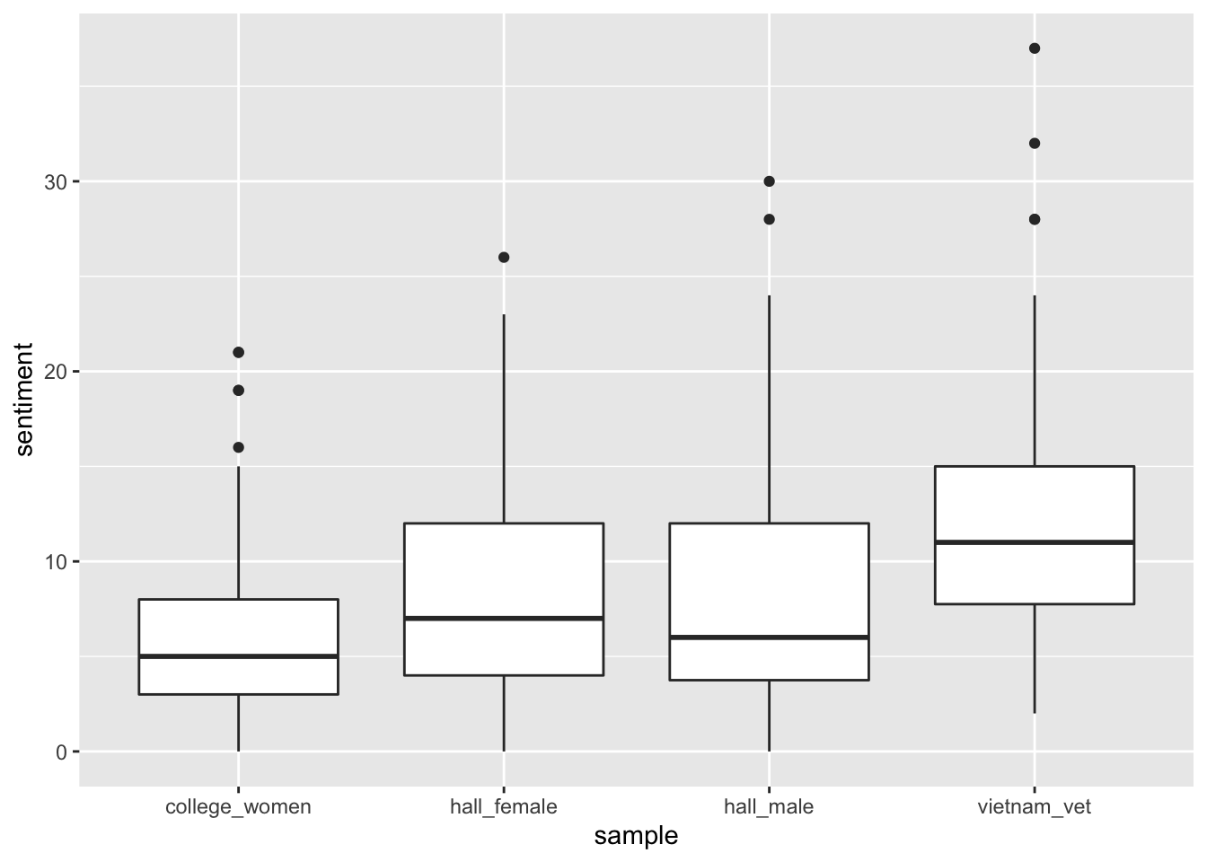
We can see that the vietnam_vet dreams appear to contain the most sentiment. In circumstances where the dataset allows us to compare the samples statistically, we could have used an ANOVA here to check whether these differences are significant. We might also want to take a look at the the single dream with the highest sentiment score. If we arrange the dataset by sentiment, in desceding order, this will give us the value.
df_sentiment %>%
  arrange(desc(sentiment))
## # A tibble: 400 × 5
## # Rowwise:
##    sample      dream_number positive negative sentiment
##    <chr>              <int>    <dbl>    <dbl>     <dbl>
##  1 vietnam_vet          165       15      -22        37
##  2 vietnam_vet          170       14      -18        32
##  3 hall_male            226       11      -19        30
##  4 vietnam_vet          113       11      -17        28
##  5 vietnam_vet          121        2      -26        28
##  6 hall_male            272       19       -9        28
##  7 hall_female          315       20       -6        26
##  8 vietnam_vet          191        0      -24        24
##  9 hall_male            279        8      -16        24
## 10 vietnam_vet          106        9      -14        23
## # … with 390 more rows
Dream number 165 has the highest sentiment score, and we can see that it contains both negative and positive sentiment. This is the benefit of our split-apply-combine approach. You can imagine that if we had simply combined our values the positive 15 and negative 22 would have resulted in total score of only -7. Let’s take a look at this dream, and see what sentiment it contains.
| dream |
|---|
| I’m young. While riding in a railroad boxcar with other people I meet a girl, a plain looking tomboy whose personality makes her alluring. The conductor explains that the center of the wooden floor is made of glass, it will not support the heater I’ve brought. No matter. I will lend it to the man who has asked to use it. One, two or three weeks at a time he can take it wherever he likes. We arrive at a summer village, which the girl belongs to. Several times, as we walk down a dirt path bordered by chicken wire, I ask if the area is safe. The girl assures me it is, and points out several dark green wooden rowboats tied up to the shore. With these, we can take lessons in a specific rowboat technique. When we sleep next to each other, we talk, and several times I choke up. It’s the war. I’m thinking how awful things can get, but I do not tell her that’s what bothers me. When we arrive at a busy amusement park there are people crowded by entrance. A woman who looks like a woman who resembles Chris D elbows the girl several times. In the slow moving melee I lose sight of the girl, who has entered the amusement park. We haven’t made emergency plans; how will I know where to look for her, or she for me? It’s as if everything is lost. However I decide to stay put and wait for her. I’m so happy when she returns. I really like this girl. She is my friend. I point out the woman who elbowed her. She seems an angry woman. Angry at life |
And as we expected this does is a dream with many of positive words (‘like’, ‘amusement’, ‘safe’) and negative ones (‘lose’, ‘angry’, ‘war’).
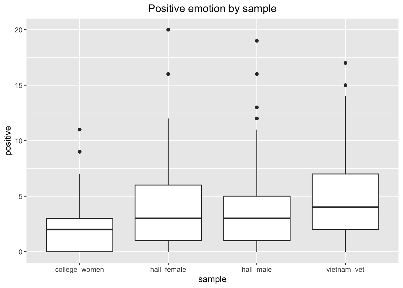
We could also compare the four samples on positive and negative emotions separately.
df_sentiment %>%
ggplot(aes(y = positive, x = sample))+
  geom_boxplot()+
  labs(title = "Positive emotion by sample")+
  theme(plot.title = element_text(hjust = 0.5))
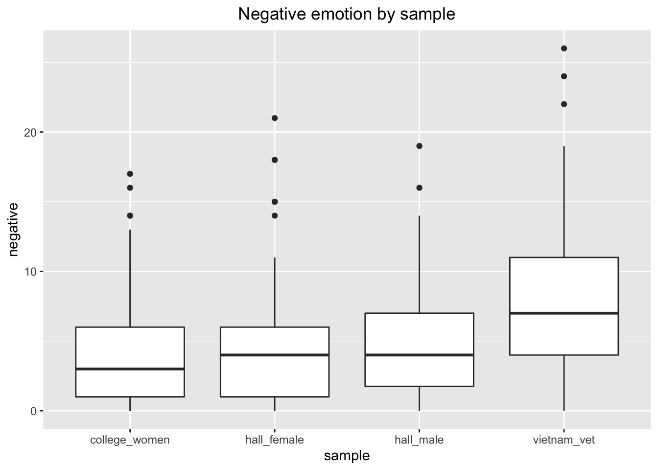
For the negative emotion, I have taken the absolute value with abs() function so that that it plots in the same direction as positive emotion.
df_sentiment %>%
ggplot(aes(y = abs(negative), x = sample))+
  geom_boxplot()+
  labs(title = "Negative emotion by sample")+
  ylab("negative")+
  theme(plot.title = element_text(hjust = 0.5))
Scatterplot of positive and negative sentiment by dream
We can plot the two sentiment vectors against one another, to see if any pattern emerges between the two sentiment scores. The alpha value (transparency) is set to .7, as many of the points overlap and increasing the transparency can aid the readability of the graph. We also add a bit of jitter to avoid overplotting.
df_sentiment %>%
  ggplot(aes(abs(negative), positive, colour = sample))+
  scale_color_manual(values = c("red", "skyblue", "orange", "darkgreen"))+
  xlab("Negative sentiment")+
  ylab("Positive sentiment")+
  geom_jitter(alpha = .5)
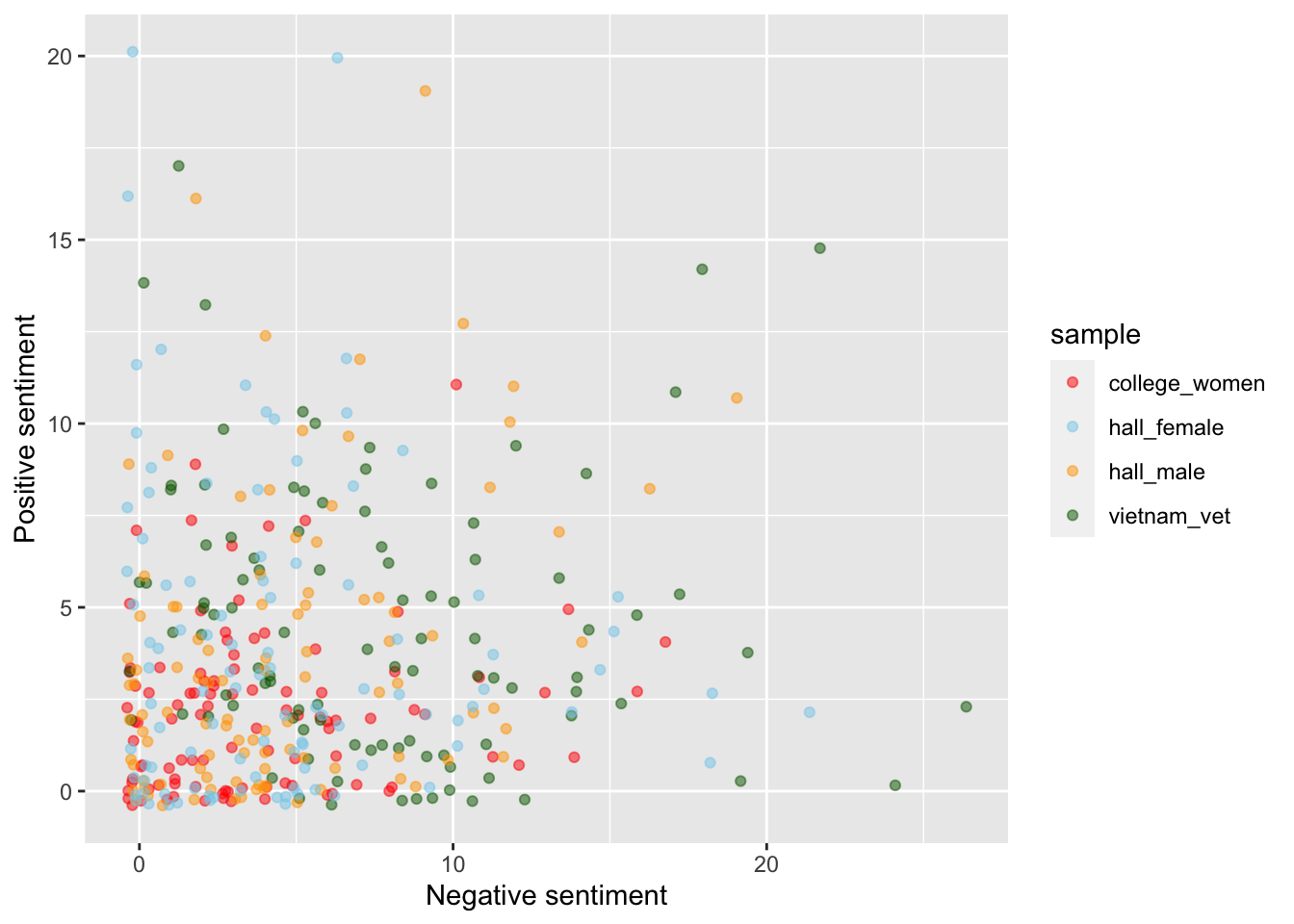
There is no clear relationship between the positive and negative emotion. Clustering close to either axis would have implied that many dreams contain high amounts of positive or negative emotion, but not both. Whereas we see quite a spread across the graph, which shows that dreams can vary across positive and negative emotions. However, uni-direction emotional dreams do occur as well. If we look up the y axis we can see a number of blue and green dots from y = 10 to = y 22 where the value for x is probably 0 (after taking account of the error introduced in the jitter). These are dreams with only positive sentiment. The same uniformity can be seen in some of the dreams represented by green dots on the x axis from x = 12 to x = 23.
Word count
We have not controlled for word count in our analysis of sentiment. It is possible longer dreams are more likely to have sentiment words in them. We could pull in the word count data from one of the previous dataframes to check this. Here we unnest the tokens from the original dataframe (df), but we don’t remove the stopwords. We then group_by the dream_number and calculate a count variable of the number of words in each dream.
df_freq <- df %>%
  unnest_tokens(word, dream) %>%
  group_by(dream_number)%>%
  summarise(count = n())
We can paste this new variable back in to our df_sentiment database with a left_join.
df_sentiment <- df_sentiment %>%
  left_join(df_freq, by = "dream_number")
We can run a quick correlation on sentiment and count to see if there is a relationship.
with(df_sentiment, cor.test(sentiment, count))
##
## 	Pearson's product-moment correlation
##
## data:  sentiment and count
## t = 9.287, df = 398, p-value < 2.2e-16
## alternative hypothesis: true correlation is not equal to 0
## 95 percent confidence interval:
##  0.3379632 0.4994153
## sample estimates:
##       cor
## 0.4220297
There is a positive correlation, so it would be sensible to convert our sentiment metric to a sentiment per word scale. We can call this “sent_prop” - short for ‘sentiment proportion’. We will also multiply by 100 to express sent_prop as a percentage of words used in each dream.
df_sentiment <- df_sentiment %>%
  mutate(sent_prop = (sentiment/count)*100)
Let’s see if this makes any difference to the distribution of sentiment across the 4 samples of dreams.
df_sentiment %>%
  ggplot(aes(x = sample, y = sent_prop))+
  geom_boxplot()+
  ylab("Percentage of sentiment words per dream")
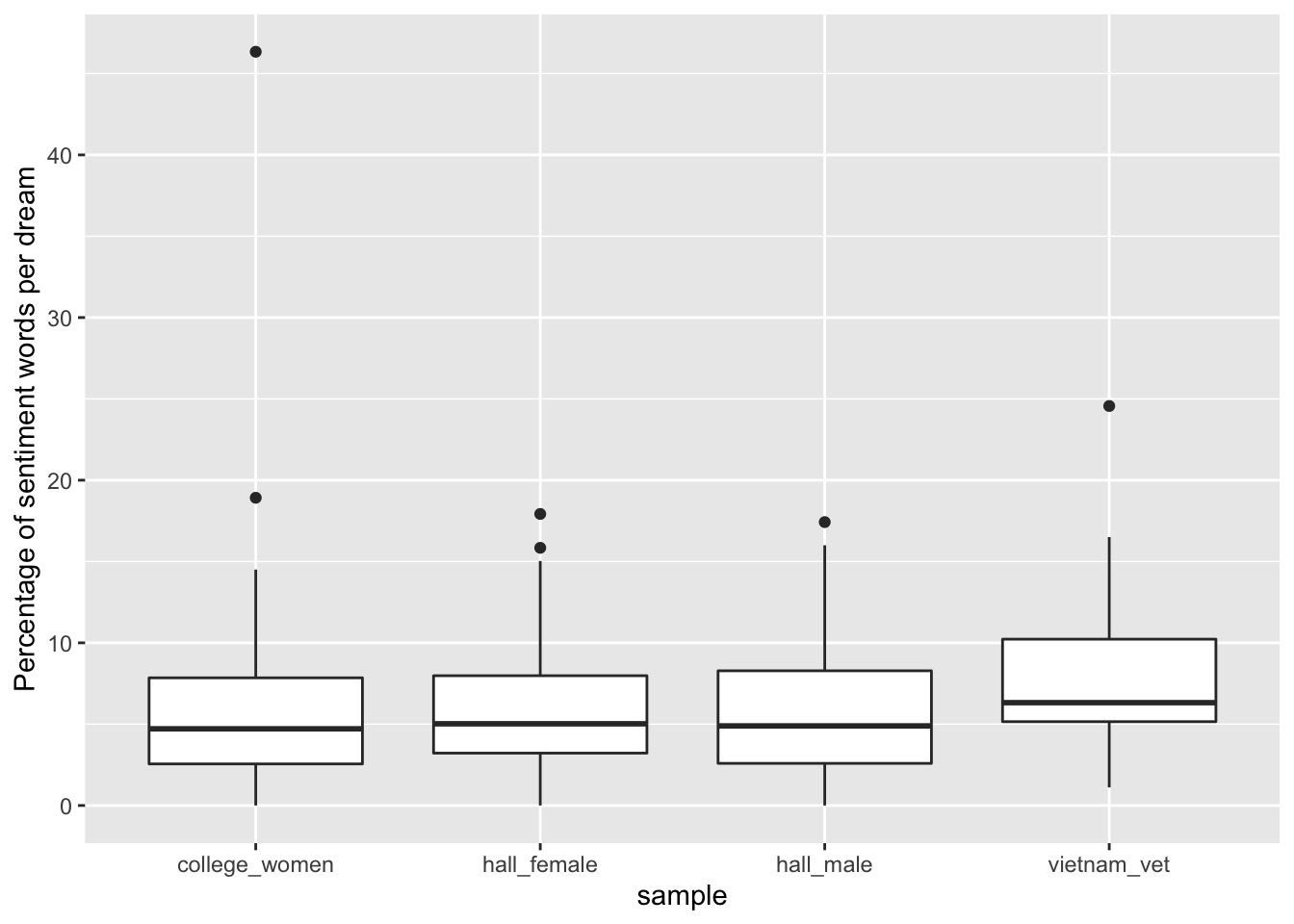
This has reduced some of the differences between the samples. We could check if the earlier difference in sentiment words between the samples was due to variations in word count by running a boxplot on our count variable.
df_sentiment %>%
  ggplot(aes(x = sample, y = count))+
  geom_boxplot()+
  ylab("Number of words per dream")
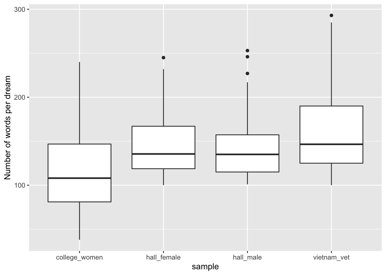
This does appear to be the case. This shows how important controlling for word count could be in comparing texts. However, the sentiment per word needs to be treated with some caution. For instance, we still might want to know why some people express both more words and more emotion, rather than less words and less emotion. Looking at the last boxplot for instance, could make you wonder, why do the college women appear to use less words to describe their dreams that the hall females? However, investigating questions such as these is beyond the scope of this post.
- Posted on:
- February 15, 2020
- Length:
- 25 minute read, 5286 words
- See Also: